Statistical Modelling of Timing Sidechannels
2. Dezember, 2021

In this blog post we present a Bayesian statistical model to detect cryptographic timing attacks. This model is one of the results of a customer embeddedhardwareassessment performed by the SCHUTZWERK GmbH. The assessment was performed in a gray box context, i.e., we were able to interact with the encryption hardware, but were not given any internal implementation details.
Background
In timing attacks on cryptographic systems, the goal is to establish a side channel via timings. This means, that not the in- and outputs of the cryptographic system are under attack, but rather some seemingly harmless information, in this case the running time of the algorithm. Based on multiple measurements of the running time the key or other secrets may be leaked.
As a simple example, consider an encryption function where the duration of the encryption operation depends on the number of zero bits in the key. While the encryption may be secure, if access is given only to the resulting pairs of plaintext and ciphertext, the additional measurement of the duration of the encryption operation decreases the key space significantly. Consequently, the key is significantly easier to recover by an attacker who has additional knowledge about the running time of the encryption.
The same attack can be applied when the duration of the encryption operation depends on the content of the plain text instead of the key. Another variation targets the decryption instead of the encryption function. Of course, this attack can also be generalized to signatures or other cryptographic primitives.
In summary, the goal of a timing attack is to distinguish between two (or more) secret states by measuring the duration of the operations handling the secrets.
Excursion: How timing attacks occur
It is surprisingly hard to implement a cryptographic algorithm in such a way that it is not vulnerable to timing attacks. The running time of the code needs to be independent of the secret inputs, i.e. of constant duration. This is in contrast to the usual requirement of optimization that is prevalent in other domains. As an example, if two strings are compared for equivalence, optimized code compares the two strings – character by character – and stops as soon as a difference is found. However, in this case the running time directly corresponds to the first difference of the strings. Thus, by measuring the duration of the string comparison algorithm, the length of the common prefix can be inferred.
A good overview of tricks used for converting common functions into functions running in constant time can be found inthiscompilation .
In the following paragraphs, we present two real-life timing attacks in AES and RSA implementations to watch out for.
AES
Consider the case of AES encryption. One step in the AES algorithm is an S-Box lookup. Naively, this is a table lookup, where the index is secret. However, when implemented as a lookup table, the implementation is vulnerable to timing attacks. Looking up entries closer to the start of the table takes less time than looking up latter entries. As the index of the table is considered secret, the running time can leak secret inputs. For a more detailed exposition see Cache-timingattacksonAES by Bernstein.
RSA
As another example, consider RSA signatures. In RSA, $m^e$ needs to be computed where $m$ is the message and $e$ is the secret key of the sender. If $e$ is “small” computing $m^e$ is fast. Whereas, if $e$ is “large” the exponentiation takes longer. If a square and multiply algorithm is used for the exponentiation, the amount of squaring operations corresponds to the amount of one bits in the binary representation of $e$.
Implementing a timing distinguisher
When transferring a timing attack from academic theory to practical assessments, there are some challenges. Remember that the goal of a timing attack is to distinguish between two (or more) secret states by measuring the duration of the operations. If only a single time measurement is taken for each state that should be distinguished, the durations are different. However, this does not mean that a timing attack is possible. Single measurements suffer from multiple sources of noise, e.g., the communication between the hardware chips is not of in constant duration. Consequently, multiple measurements can be created and the deviations can be filtered out, e.g., by averaging. However, averaging does not take into account the distribution of the noise. And the averages of the measurements of both setups still differ. The more measurements are taken, the more certainty there is in the result. But how many measurements are sufficient?
As a solution to this challenge, we implemented a Bayesian distinguisher that returns the certainty that the implementation suffers from a timing attack. Our distinguisher takes two lists of timings as an input and returns the probability that these lists are sampled from the same distribution.
A similar solution can be accomplished by the Kolmogorov-Smirnov (KS) test. However, while the KS test makes fewer assumptions on the distributions than our test, it only returns a qualitative statement, i.e., whether the samples are from the same distribution or not, without considering probabilities. The result of the KS test is a p-value which is often misunderstood. Additionally, it does not allow any introspection into the data model. In contrast, our implementation returns the probability for the samples stemming from the same distribution and therefore the certainty of the vulnerability to a timing attack.
Generation of test data
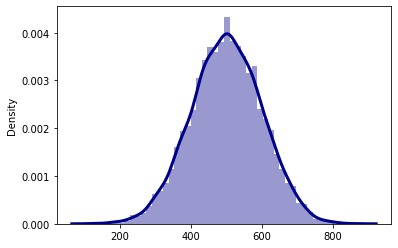
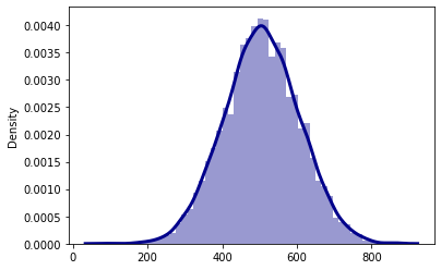
As we cannot disclose the real data of the assessment due to a non-disclosure agreement we artificially generate test data in order to present our approach. Let us assume that we measure the duration needed for the encryption operation. First, we measure the durations required for encryption with a key key1 5000 times. Next, we measure the duration of the same encryption with a different key key2 5000 times. The durations are samples from a Gaussian distribution with a mean of 500 and 505 respectively, and standard deviations of 100, each.
from scipy import stats
import numpy as np

key1_durations = stats.distributions.norm(loc=500, scale=100.0).rvs(size=5000)
key2_durations = stats.distributions.norm(loc=505, scale=100.0).rvs(size=5000)
import seaborn as sns
sns.distplot(key1_durations, kde=True,
             color = 'darkblue',
             kde_kws={'linewidth': 3})
sns.distplot(key2_durations, kde=True,
             color = 'darkblue',
             kde_kws={'linewidth': 3})
Bayesian Data Model
For our Bayesian analysis a data model needs to be specified first. Assumptions about the measured data and their distributions need to be created based on the use case. In a next step, the parameters of the data are inferred.
In our data model, the means of both distributions that are compared are chosen from a Gaussian distribution. Note that we are cheating here. As we sampled the test data from a Gaussian distribution, we already know that such a distribution will fit. Nevertheless, a Gaussian distribution makes sense in our use case independent of our knowledge about the test data. There are multiple sources of noise which affect our measurement. Thus, due to the central limit theorem, this results in a Gaussian distribution given a “large enough” number of noise sources.
More accurately, we assume that the measured durations are distributed with mean $\mu$ and standard deviation $\sigma$. As these parameters are unknown, we treat them as random variables from a prior distribution. The parameters of the prior distribution are then inferred using Bayes’ theorem and state-of-the-art Markov Chain Monte Carlo methods. Note that this is in contrast to a frequentist analysis, where only the parameters with, e.g., the highest likelihood, are inferred. In a Bayesian model, such as the one presented here, the parameters are sampled from a distribution distribution themselves.
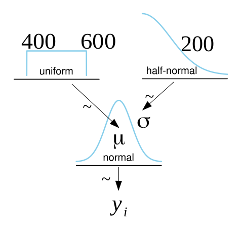
We choose $\mu$ from the uniform distribution in a sensible range, i.e., between 400 and 600 as we do not have any prior knowledge of the real $\mu$. We choose the deviation $\sigma$ from the Half-Normal distribution with a mean of zero and a standard deviation of 200. Basically, the Half-Normal distribution is the positive side of a normal distribution. This makes sense, as we do not expect $\sigma$ to be particularly large. 200 is just chosen as a high number to fit with our expectations.
Our data model is very similar to the model of Kruschke (Bayesian estimation supersedes the t test. J Exp Psychol Gen. 2013;142(2):573-603. doi:10.1037/a0029146), but easier to work with. Kruschke makes use of a Student’s t-distribution, which is less sensitive to outlier observations than our Gaussian distribution.
Formally our data model looks as follows:
$$ \begin{aligned} \mu &\sim Uniform (400, 600) \\ \sigma &\sim \lvert N(0, 200)\rvert \\ y &\sim N(\mu, \sigma) \\ \end{aligned} $$
Here, $y$ denotes the data. Our Bayesian data model can be visualized using a Kruschke diagram.
As a next step, the parameters need to be inferred. This is done using a Markov-Chain Monte Carlo algorithm (MCMC). In particular, we are using PyMC3, which implements state-of-the-art MCMC algorithms such as the No-U-turn sampler. This is a variant of the Hamiltonian Monte Carlo algorithm, where the step lengths are determined dynamically. For learning more about MCMC algorithms we recommend starting by learning the Metropolis-Hastings algorithm as that is conceptually the simplest one and the starting point for many of the modern improvements.
Using PyMC3 we compute the posterior distribution of the parameters and visualize them accordingly. More exactly, we can draw samples from the posterior distribution. Given enough samples, it is possible to approximate the distribution. As we are dealing with two sets of measurements, we can compute the difference of the distributions of their means.
import pymc3 as pm
import pandas as pd

with pm.Model() as Model:
    μ_1 = pm.Uniform ('μ_1', lower=400, upper=600)
    σ_1 = pm.HalfNormal('σ_1', sd=200)
    y_1 = pm.Normal('y_1', mu=μ_1, sd=σ_1, observed=key1_durations)
    μ_2 = pm.Uniform ('μ_2', lower=400, upper=600)
    σ_2 = pm.HalfNormal('σ_2', sd=200)
    y_2 = pm.Normal('y_2', mu=μ_2, sd=σ_2, observed=key2_durations)
    diff_of_means = pm.Deterministic('diff_of_means', μ_1-μ_2)
    diff_of_std = pm.Deterministic('diff_of_std', σ_1-σ_2)
    trace = pm.sample(1000)
After sampling from the posterior distribution, convergence needs to be checked. Note that this is about convergence in distribution instead of convergence to a single value. In order to check convergence, the trace is plotted. If the traces are meandering, i.e., the latter samples visually depend on the previous samples, the convergence is not good. Intuitively, if the next samples are heavily correlated with the previous samples, the convergence is not given. However, this only provides an intuitive explanation, as MCMC algorithms always return correlated samples.
import arviz as az
az.plot_trace(trace)
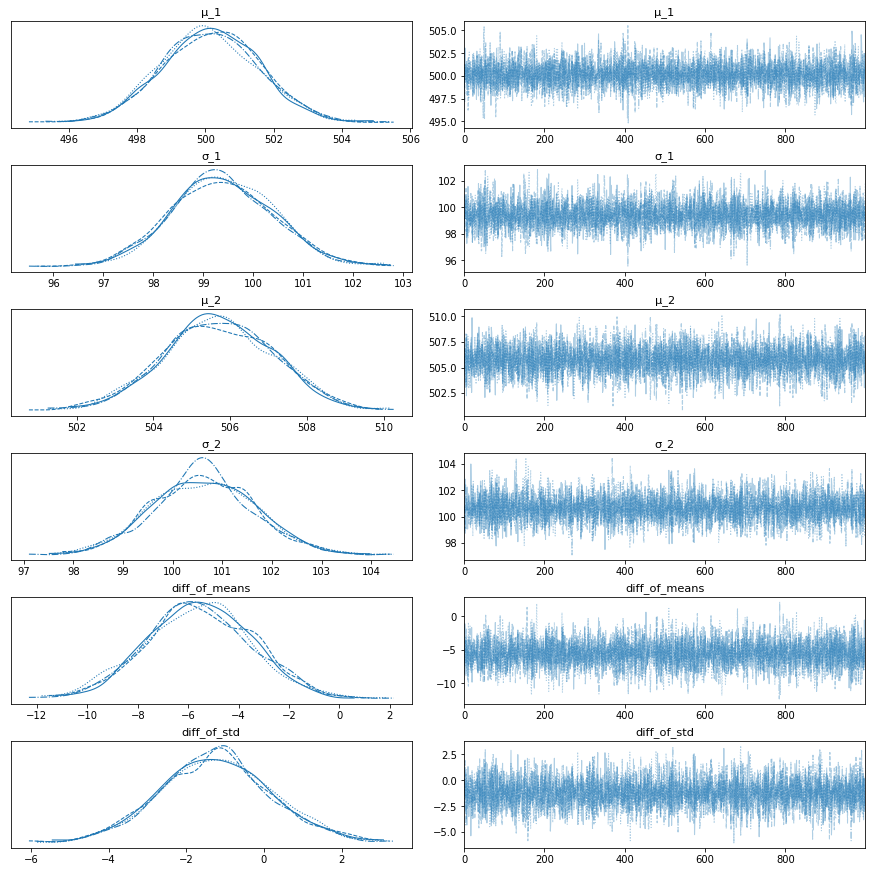
As we can see, the traces converge, as there are no obvious meandering patterns. Next, we plot the posterior distributions of the means, the standard deviations, and their differences.
az.summary(trace)
| mean | sd | hdi_3% | hdi_97% | mcse_mean | mcse_sd | ess_bulk | ess_tail | r_hat | |
|---|---|---|---|---|---|---|---|---|---|
| μ_1 | 500.152 | 1.426 | 497.573 | 502.843 | 0.017 | 0.012 | 6688.0 | 3258.0 | 1.0 |
| σ_1 | 99.398 | 1.020 | 97.369 | 101.157 | 0.012 | 0.009 | 6765.0 | 3006.0 | 1.0 |
| μ_2 | 505.714 | 1.434 | 503.124 | 508.460 | 0.017 | 0.012 | 7214.0 | 3384.0 | 1.0 |
| σ_2 | 100.631 | 1.019 | 98.778 | 102.627 | 0.013 | 0.009 | 6451.0 | 3159.0 | 1.0 |
| diff_of_means | -5.562 | 2.075 | -9.333 | -1.557 | 0.026 | 0.020 | 6471.0 | 2896.0 | 1.0 |
| diff_of_std | -1.233 | 1.429 | -3.773 | 1.667 | 0.018 | 0.018 | 6553.0 | 3022.0 | 1.0 |
az.plot_posterior(trace)
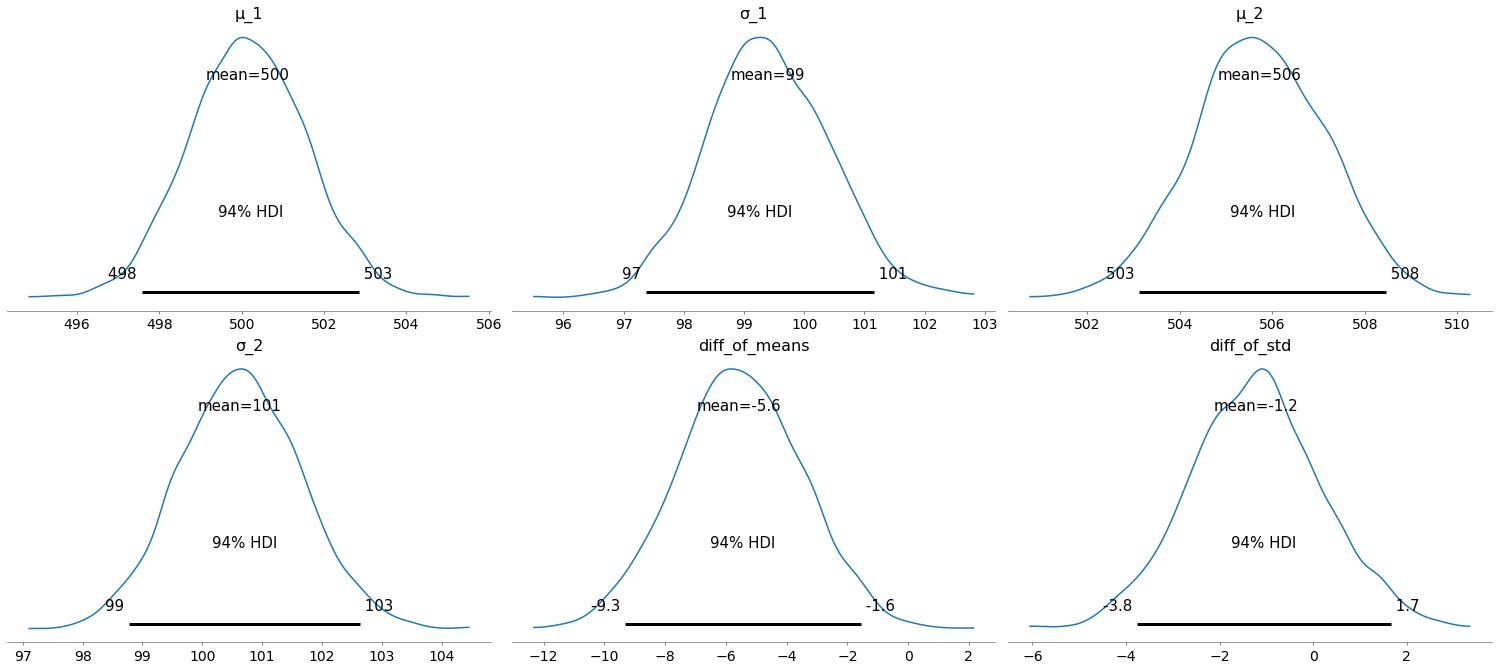
The 94% HDI is the 94% highest density interval. This corresponds loosely to confidence intervals. With 94% certainty the real (estimated) value is inside the 94% HDI.
We can see that the HDI of the means $\mu_1$ and $\mu_2$ do not overlap. From the diagram at the bottom center we know that with a certainty of 94%, the difference of the means is between -9.3 and -1.6. As this interval does not contain zero, we can conclude that the data is indicative of a timing attack with more than 94% probability.
Summary
In summary, we provided a statistical approach that allows to detect the susceptibility of a black box cryptographic implementation to timing attacks given several timing measurements. Additionally, our approach does not produce a qualitative statement, but instead a quantitative one, i.e., the certainty of the timing attack is returned depending, e.g., on the amount of performed measurements.
Finally, to prove our claims, we implemented our model utilizing Python and showed its feasibility using generated test data.
References
- Title picture: Photo by TimaMiroshnichenko from Pexels .